[Devember 2021] Tools for working with 3D volumes of biological data

I’m pursuing a PhD in the field of structural biology. I’ve posted about it here before, (that thread is due for an update) but my university recently took possession of a large expensive microscope that is used to image small molecules like proteins, DNA, RNA, as well as larger biological assemblies such as viruses and cells. I’m currently responsible for the day-to-day operation of this microscope, as well as the computing infrastructure surrounding it, which is quite extensive.

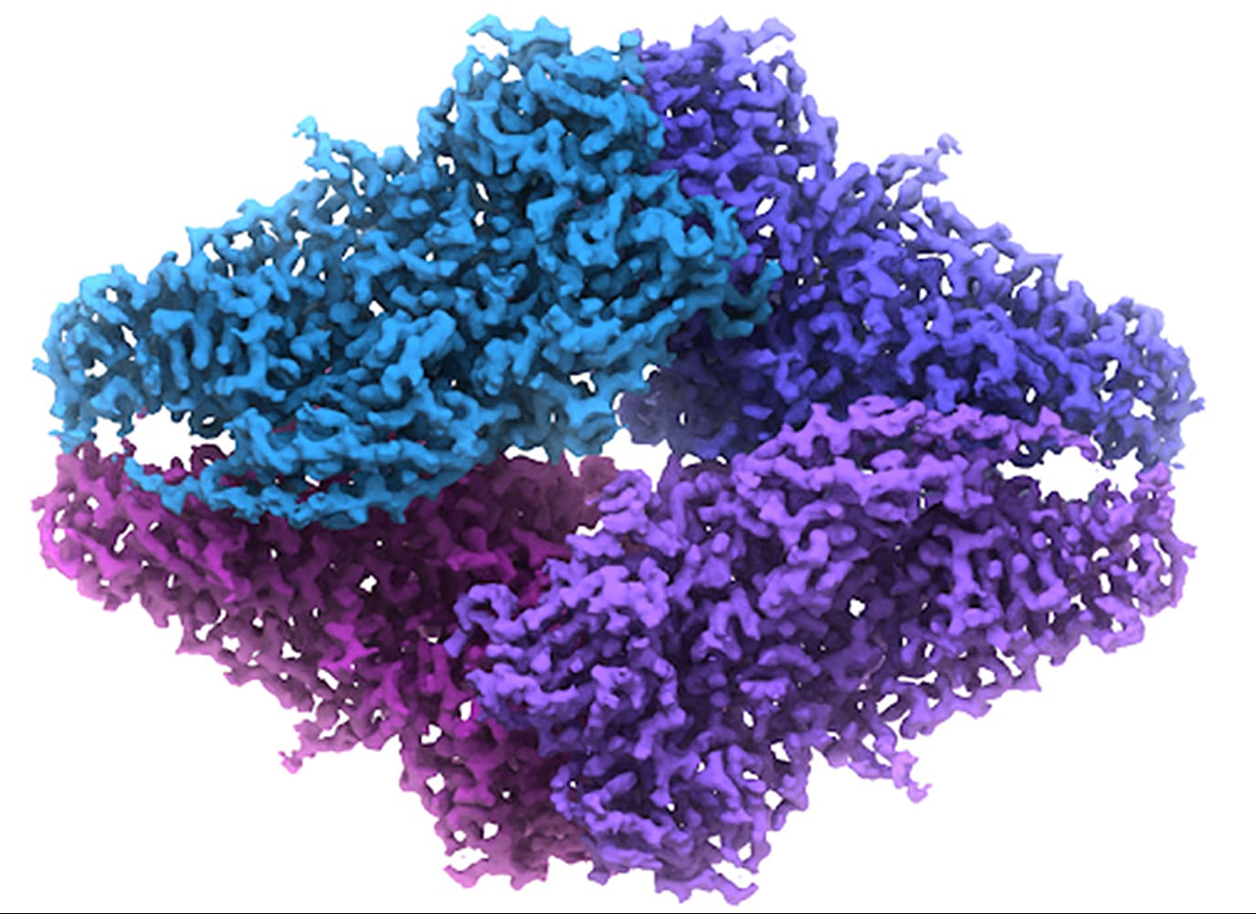
Experimental data in this field generally consists of a file that maps electron density to Cartesian coordinates at some specific pixel spacing, where the pixel spacing is representative of some distance in Angstroms or nanometers. It is, to my knowledge, always cubic. So at the end of the process of collecting and refining data of a protein, I might end up with what we call a “map” or “volume” that is essentially a 3D array of some size (say, 100x100x100) at some specific pixel spacing (say, 2.0 angstrom). That would mean I have a cube that is 200 cubic angstroms, and any position on a lattice in that cube has a corresponding value that represents the density of a pixel (or voxel) there.

Here is a 2D projection of what that looks like:

Then, if we know the amino-acid sequence of that protein, we can “build” it into that density, using rules we know about the shapes, sizes, bonds, angles, etc, of amino acids and peptides. The higher resolution the 3D map, the more confident we can be about the atomic model we build into it, and the more fine details we can model.

Here is an example of a protein atomic model being built into a 3D density map:

image

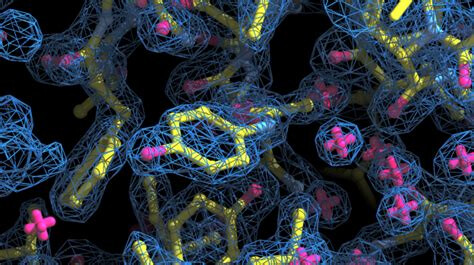
In this image, the map is the blue mesh, and the atoms and bonds are represented by the red (oxygen) and yellow (carbon).

In the old days of structural biology, the data coming from traditional methods was generally lower resolution. This means that to see a certain level of details that are only visible at higher resolutions, various techniques had to be employed to existing data to squeeze the maximum amount of information out of it. Some of these strategies were:

  • Averaging data that had symmetry to improve the signal to noise. If you have data that has, say, 4 fold symmetry, you can expect real density to self-reinforce while noise will self-cancel (unless it’s systemic noise, but there are other strategies for dealing with systemic noise).
  • Solvent flattening (fitting peaks to solvent in fourier space to help “sharpen” the map and distinguish between protein and non-protein density which allows for a less ambiguous fit)
  • Masking and thresholding, which again rely on the fact that you can expect ordered regions to be your molecule of interest, and less-ordered regions to have lower density thresholds.
  • High and low pass fourier filtering, which excludes wavelengths of specific frequencies to try and remove noise
    …as well as a bunch more.

As the field of x-ray crystallography grew with the development of Synchotron beamlines that allowed for higher-resolution data collection, and the invention of CMOS image sensors in cryo-EM which also allowed for the collection of higher-resolution data, these strategies became less frequently used. As such, many of the people that developed and maintained the software for these techniques either moved on to other jobs, or retired and haven’t been replaced. In particular, the biggest loss was the Uppsala Software Factory software, which was a collection of tools for working with and manipulating 3D volume data to do all sorts of things with it. The tools hadn’t been updated since the early 2000’s, and last year, the main website, including all the documentation, went down.

This would be OK, because with high resolution data, they aren’t needed anymore, except that we have another exciting development in the field of structural biology that has actually made them quite useful: tomography.

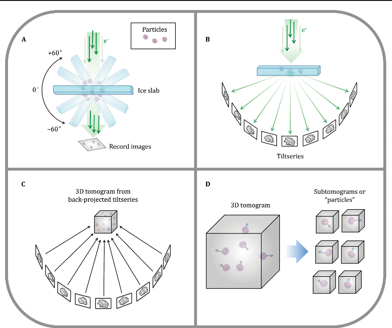
While traditional structural data comes from imaging and classifying hundreds of thousands or millions of highly pure, homogenous particles over the course of weeks, and constructing that into one final model, tomography is a technique that lets us look at a single particle, but from multiple angles, and then combine those angles in fourier space to construct a 3D volume. However, because we are exposure limited (send too many 200 kV electrons at the same particle and it will degrade), the quality of this data tends to be of lower resolution.

One thing we can do, however, is extract particles from the 3D volume, and average them either together with other particles, or “locally”, to find symmetry on themselves and take advantage of that to increase our resolution.

As I’ve been working with more and more low-resolution tomographic data, I’ve been lamenting the fact that the traditional tools for squeezing information out of low-resolution data, and manipulating and working with 3D volumes.

While the binaries themselves, and the source code, are present on GitHub (GitHub - martynwinn/Uppsala-Software-Factory: These are the famous Uppsala Software Factory programs, rescued into GitHub.), I’ve been unable to re-compile them as I know nothing about Fortran, and also, they are having a hard time with modern file formats for this type of data. I’ve written a couple of tools and scripts to make modern file formats compatible, but as what I’m trying to do is becoming more complex, that solution is failing rapidly.

My goal, then, is to begin to re-write/re-implement these tools in Python or another more-modern language, and to eventually release a full package capable of doing the bulk of the operations that these tools used to do. I’m terrible at math, and I’m terrible at programming, so I am going to recognize right now that this is a huge undertaking that will likely take me years, if it ever does succeed.

Therefore, for my Devember project, my goal is going to be more simple:

  1. I want to develop a tool that will re-orient a 3D volume to be centered on its origin. Most modern software outputs these volumes so that their origin is 0,0,0 (the bottom left). I want to develop a tool that will move that origin to be the center of the volume. So that if you have a 100x100,100 volume, the origin is 50,50,50. This is because for averaging, it is much easier to assume that the origin is the center of the volume, and then to average symmetrically around that origin.

  2. I want to develop software that is capable of displaying a 3D volume in 2D slices, and pan through those slices on any of the X, Y, and Z axes

and…

  1. (stretch goal) is to develop a rudimentary radial averaging program that will at least generate symmetry operators for some angle theta and average a 2D plane of a matrix and report a correlation coefficient. I’m not expecting to get this done yet, but I would be thrilled to at least have a prototype by Jan. 1st.

Also unstated is a way to open and work with these files, as that’s a necessary pre-requisite to doing any of this.

8 Likes

1st Update:

The anatomy of an MRC file

3d maps are stored in .ccp4 files, and later on .mrc files (which are functionally identical). The .ccp4 files were initially from the Collaborative Computational Project. CCP4 was initially for X-ray crystallography, and eventually the file format was revamped by the Medical Research Council in the UK to be better suited to electron microscopy data in the year 2000. In 2014 it was revamped again to allow an extended header to hold more metadata and other important information. Header information includes things like pixel spacing (i.e. something that translates pixels to equivalent angstroms or nanometers), value scaling information, size, etc.

One of the issues I’m running into is that a number of the tools I’m using haven’t been updated since the early 2000s, and therefore aren’t compatible with the .mrc 2014 format entirely. Sometimes, reading in the files crashes them, somewhere in the header.

The files are hexadecimally encoded, and the 2014 file format specifications are here:

https://www.ccpem.ac.uk/mrc_format/mrc2014.php

Beyond the header (bytes 1-1024), is the data block. As far as I can tell, the data block can be as large as needed to hold the data. The datablock is a 3D matrix. Each value in the matrix corresponds to some scaled value of electron density. When I take an image with the electron microscope, what I’m actually recording are electrons impacting the camera sensor. That number is called “counts”. With modern cameras, we can actually come pretty close to detecting individual electron impacts. That counts number is then recorded basically like a bitmap (excepted it’s not always scaled), and when reconstructed into 3D, the value in the matrix tells the electron density at that position, while the location in the matrix tells the location of that position in 3D.

Interacting with an MRC file
I don’t want to work in hexadecimal. While the documentation is excellent, and I’ve worked in hexadecimal before trying to figure out why things are crashing (it’s always bytes 97-196 it feels like), there is thankfully already a Python library for working with .mrc files, aptly named…mrcfile:

In addition to a couple of handy functions builtin, essentially what mrcfile does is it converts the hexadecimal in the header to ASCII, and it converts the hexadecimal in the data block to a NumPy matrix. This means I can open the files in Python, work with them using NumPy and other Python libraries, and save them again as an MRC file when finished. This should greatly reduce the effort needed for this project.

There are three dependencies that I can tell:

import sys, mrcfile, numpy as np

Next I need to open the file. I’d like to pass the file from the command line, so I came up with:

with mrcfile.open(str(sys.argv[1]), mode='r+') as mrc

I’d appreciate it if anyone had any suggested reading on command line arguments with Python. In this case, per the documentation, ‘r+’ opens the file in r/w mode.

Next I want to print the header information in ASCII, and an ASCII representation of the data block NumPy matrix. There is an object property for header that looks promising, so I can try that, and similarly I can do the same for data.

My final code looks like this:

import sys, mrcfile, numpy as np

with mrcfile.open(str(sys.argv[1]), mode='r+') as mrc:
    print(mrc.header)
    print(mrc.data)
    mrc.flush()

in this case, mrc.flush() writes changes to the disk and closes the file.

Running python3 print.py tmp.mrc results in:

(200, 300, 200, 2, 0, 0, 0, 200, 300, 200, (900., 1350., 900.), (90., 90., 90.), 1, 2, 3, 42.864872, 248.33524, 162.26773, 1, 0, b'\x00\x00\x00\x00\x00\x00\x00\x00', b'', 0, b'\x00\x00\x00\x00\x00\x00\x00\x00\x00\x00\x00\x00\x00\x00\x00\x00\x00\x00\x00\x00\x00\x00\x00\x00\x00\x00\x00\x00\x00\x00\x00\x00\x00\x00\x00\x00\x00\x00\x00\x00\x49\x4D\x4F\x44\x00\x00\x00\x00\x00\x00\x00\x00\x00\x00\x00\x00\x00\x00\x00\x00\x00\x00\x00\x00\x00\x00\x00\x00\x00\x00\x00\x00\x00\x00\x00\x00\x00\x00\x00\x00\x00\x00\x00\x00', (100., 150., 100.), b'MAP ', [68, 65,  0,  0], 17.094187, 1, [b'Written by PEET / MatTomo 22-Apr-2021 09:26:35                                  ', b'', b'', b'', b'', b'', b'', b'', b'', b''])
[[[162.61371 133.7904  131.44235 ... 156.04503 166.31416 175.38896]
  [162.61371 134.77493 133.61285 ... 155.44954 157.5272  164.20723]
  [162.61371 135.52399 139.91861 ... 160.28831 154.85309 155.89516]
  ...
  [160.95091 156.39767 156.10796 ... 189.18652 202.2494  210.65956]
  [159.98395 153.40433 151.55235 ... 161.23901 171.87277 181.64807]
  [166.53502 160.05673 155.40648 ... 145.8512  146.06181 155.96167]]

 [[143.44464 134.8575  127.22648 ... 170.83243 176.72656 178.22858]
  [150.28072 139.2749  131.64488 ... 172.5024  173.89108 174.33745]
  [151.67004 143.40686 138.8311  ... 175.78445 171.21962 166.52661]
  ...
  [164.2355  162.09772 160.41669 ... 182.94122 185.95598 183.1842 ]
  [163.80745 158.60977 157.27316 ... 161.44473 166.44623 169.63568]
  [165.81233 159.66911 158.13333 ... 148.64095 148.43239 153.57199]]

 [[146.56082 139.24031 132.22955 ... 186.4479  188.11671 185.07533]
  [160.51132 150.1365  137.99564 ... 183.31944 187.73503 189.46342]
  [164.17575 154.48367 146.81454 ... 182.27373 181.27708 177.36957]
  ...
  [168.47905 171.2478  169.32349 ... 174.77365 169.53305 157.81972]
  [171.29181 169.30852 167.28891 ... 162.54257 161.87354 156.53036]
  [170.98503 167.1167  165.44217 ... 151.30786 150.61195 152.7901 ]]

 ...

 [[168.45381 157.58435 151.54663 ... 172.18178 172.23207 176.38858]
  [173.86557 166.39969 162.0009  ... 146.72133 148.7712  160.17076]
  [171.431   168.52255 165.4768  ... 141.06406 147.10681 156.06792]
  ...
  [163.      163.      163.      ... 192.7547  195.77583 191.54175]
  [163.      163.00002 162.99998 ... 198.28336 206.89825 198.69138]
  [163.      162.99998 163.      ... 191.62312 192.63992 183.4547 ]]

 [[163.97047 152.12363 145.71553 ... 165.44347 160.71799 161.6005 ]
  [173.40633 160.95761 151.00027 ... 143.83438 143.04729 145.09822]
  [177.68735 167.76009 156.9156  ... 143.41397 139.13055 143.69751]
  ...
  [163.      163.      163.      ... 181.1156  192.23433 199.7037 ]
  [163.      163.      163.      ... 190.87585 203.8085  207.98398]
  [163.      163.      163.      ... 193.92291 202.4862  204.72751]]

 [[162.61371 147.93631 138.39818 ... 170.65265 166.5719  161.49603]
  [172.4552  159.0966  143.94698 ... 151.52254 148.32602 147.64355]
  [185.96162 172.562   157.3432  ... 145.16893 146.32784 148.15042]
  ...
  [163.      163.      163.      ... 161.21515 176.59705 193.64203]
  [163.      163.00002 162.99998 ... 171.32726 185.47574 199.53555]
  [162.61371 162.61371 163.      ... 187.195   196.1833  197.2368 ]]]

This is pretty close to what I need. There’s still some hexadecimal in the header (extended header) and there’s some formatting discrepancies, but this will at least get me the data and I can start working with it that way.

https://docs.python.org/3/library/argparse.html

1 Like

Hi, fellow grad student, MS in Computer Science, Machine Learning here. I don’t know anything about the biology domain but I am pretty proficient in python/numpy. There’s not much code commentary I can give since I just have periphery knowledge, not sure if these 2 points will be helpful or confusing,

  1. Again, I don’t know anything about MRC files but it seems you’re expecting some n-dimensional representation. You may have a complete understanding of the numpy output you posted so maybe my point is moot. Specifically, it’s not clear to me what the shape of the numpy output you’ve posted is (since it seems to have been truncated), but the printout of mrc.header information looks like a shape of some crazy dimensions. So it might be worth verifying the library is doing the header conversion correctly and if you need to do np.reshape to fix the dimensionality of the values in mrc.data (if you haven’t checked already).

  2. MRC files look pretty complicated for the information they hold, but if that’s the standard the bio field works in then you can also ignore this suggestion. In my opinion, numpy vectors are intuitive and easy to manipulate, and you already have a library to go from numpy back to MRC so I would suggest keeping numpy as your intermediate data structure and only converting to MRC when you are forced to. One example of flexibility: numpy vectors also can become Pytorch Tensors in case you wanted to try out another form of modeling. In the future if you feel comfortable with python’s file I/O I suggest storing your numpy vectors in HDF5 to work around any dogmatic issues with future MRC formats.
    Installation — h5py 3.5.0 documentation

1 Like

Two astute observations - thanks for the input!

My understanding is that the dimensionality is deliberately vague. The first three values in the header are actually nx, ny, and nz, so it should be 200x300x200 (i.e. a rectangle with a long axis standing on its head). The 90,90,90 tells me that the volume is cubic (90 degree cell angles).

There is a concept in the space (this may be a common computer science concept, I’m not sure) of “slow, medium, and fast” axes. This is actually something that has caused me a lot of headache in the past, but it seems to be too ingrained with the current software to really leave in the past. Because computers were slower, and you may not be visualizing the entire volume all at once, the question was: do you want to read your array into memory by row, column, or some variation? It’s not a topic I understand enough to really explain (at least not right now) but I think this article gets into it fairly well:

This isn’t really an issue with arrays of the size I’m working with now. But it’s an artifact of an older time in computing that hasn’t quite been shaking yet. Anyways, the long answer is when not truncated, the array does seem to make sense (for now). I’ll have some 2d images up in the next update I think.

There’s been some push to HDF in the field, specifically in one program that isn’t hugely used yet. Another program supports it for interoperability, but can’t write it annoyingly. MRC is annoying, but the bottleneck is unfortunately the actual software that drives the instruments records everything into MRC (and often saves excess metadata in a “.mdoc” file associated with it by name). In the interest of not biting off more than I can chew, I’m going to pretend HDF doesn’t exist for now, and if I ever get to any complicated functions, I probably will look into the switch.

One of the things that I’m trying to figure out is how to format rotation and translation matrices in an intuitive way, and I think HDF is probably a reasonable answer for that as well.